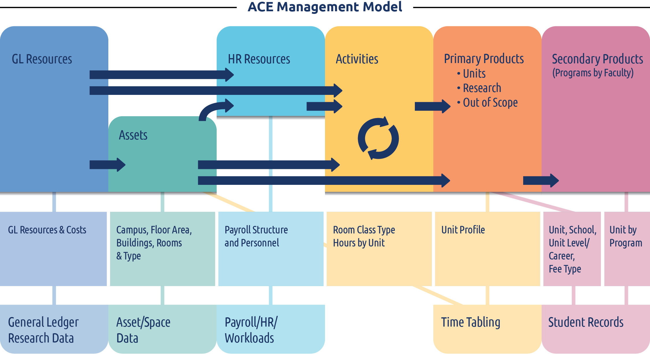
The US Higher Education Demonstration Model as a
window on Pilbara’s academic resource management solution.
Our analysis journey begins with a quick overview of the model. The model is a holistic model, that is, it covers the entire university, and includes all outputs – teaching, research, commercial, community service. The teaching outputs include all Programs and all Courses, all the way down to a course instance, which includes the where, when and how for each time the course is taught.
The model includes data from five major source systems – Finance, Asset Management, Payroll/HR, Time Tabling and Student Records. This means that once the model is built it contains all of the data required for a wide range of analysis including identifying courses for redesign or elimination, identifying programs for investment or disinvestment, analyzing workload profiles, calculating marginal costs, assist in setting pricing, identifying teaching/research relationships, scenario planning etc. Please see this blog post for a rundown of a range of different types of analysis that can be performed in the model.
Some Details about the
US Higher Education model
- 5 major source systems
- 1,600 Programs
- 3,400 course instances (when, where and how taught)
- 1,800 Rooms
- 1,300 FTE
- 5,200 finance line items
- 4.2 million rows of data for reporting


Budget decisions rarely focus directly on programs but their consequences for programs can be very important. It’s the programs that present the institution’s face to the educational marketplace.
Changes in student demand for programs affect the courses that deliver educational content, which has knock-on effects for faculty workload, facilities utilization, and margins in the departments that teach the courses. Budget decisions deal with the latter factors, which link them indirectly but consequentially to the configuration of, and demand for, programs.
In this worked example we will delve into the details of program and course costs and margins to support academic resourcing decision makers to either invest or disinvest in programs or are there more nuanced fixes that can be applied to ensure a program is financially self-sufficient.
Please note all these reports are live, so after this worked example you can go back and change filters, select different schools, programs and courses to see what you can uncover.
Universities should review summary data on program enrollment, revenue, cost, and margin during the annual budget process, just as they do for departmental data.
The report shown here carries this a step further by showing how the data can be broken down according to whether a program’s margin, etc., are generated within the school that houses its major or by other schools.
Let’s see what happens when we filter on one particular school – the School of Engineering and Comp Sciences.
Select School of Engineering & Comp Sciences
When filtered on the School of Engineering and Computer Sciences, as expected there is significant revenue and expenses associated with the school. But there is also quite a lot of revenue and expense coming from the College of Arts and Sciences, this is because that College teaches general education and certain introductory courses for Programs in Engineering and Computer Sciences.
Tip – If you hover your mouse over each of the bars in the chart above it will tell you the actual amounts.
Student demand is best understood at the program level whereas budgeting focuses mainly on departments. This disconnect has made it difficult to incorporate program-related considerations into budgeting except in the relatively rare cases where a program is being deliberately upsized or downsized. This is unfortunate, because significant consequences of many budget decisions are felt at the program level. Our model can mitigate this problem by connecting the dots between programs and courses.
The reverse is true. If you scroll down and select Biology 150 : (Campus 1, USA – Spring) – In-Person in the table below you will see only those Programs that have that course in them in the table above.
You can see that Biology 150: (Campus 1, USA – Spring) – In-Person is losing around $94 per credit hour. You can do further analysis on this course to find out what are the contributing factors. This can be used in conversations with the curriculum committees for both Biology and Life Sciences to learn the consequences for student progression. It’s likely that the 8 credit hours from the BS in Psychology represents elective-taking, in which case elimination of the instance would be less consequential. All the other ways of using course-level data are applicable here as well—for example, program margins might be improved by redesigning low-margin courses with large enrollments. These represent just two applications of the triangulated data, but it’s clear that others will emerge as users become familiar with the crosswalks between the courses and programs.